


Summary
DNS tunneling is a critical security threat where malicious actors exploit the Domain Name System (DNS) to exfiltrate data and bypass network security controls by embedding unauthorized communications within legitimate DNS queries. This blog presents Infoblox’s machine learning-based detection system that achieves 99.9 percent precision, 99.5 percent recall and a 99.7 percent F1 score in identifying DNS tunneling attacks, which, to the best of our knowledge, is the highest performing DNS tunneling detection system.
Our patented approach combines a convolutional neural network (CNN) autoencoder that generates a reconstruction loss feature with novel statistical and linguistic features extracted from DNS traffic patterns. The autoencoder learns normal DNS query behavior from millions of legitimate domains, producing reconstruction loss values that effectively distinguish between normal and anomalous activity. Our feature engineering captures many characteristics such as query frequency patterns, subdomain entropy, word segmentation ratios and payload size distributions. These features are then processed by a Random Forest classifier for final detection. This system operates in real time on billions of DNS queries daily with low false positive rates, enabling us to automatically block DNS tunneling attempts while preserving legitimate network traffic. Portions of this work were previously presented at CAMLIS and Flocon.
Introduction
The DNS translates domains (www.google.com) to resource records that contain critical information such as IP addresses (8.8.8.8). Generally, a client requests a local recursive DNS server to look up the address on its behalf. See Figure 1 for a visual explanation.
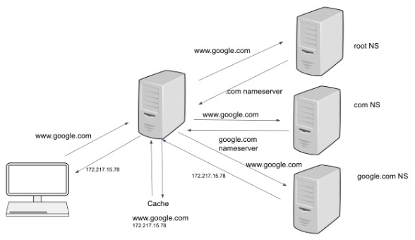
Figure 1. The typical process of how DNS operates
DNS tunneling abuses this legitimate process by creating a covert communication channel that transmits unauthorized data through DNS queries and responses—far beyond DNS’s intended purpose as defined in the RFC specifications. Since DNS traffic is typically allowed through firewalls and often goes unmonitored, attackers exploit this trusted protocol to bypass security controls and establish command-and-control (C2) channels.
Recent threat campaigns have demonstrated the growing sophistication of DNS tunneling attacks, including operations like Decoy Dog, Saitama and DNS Anchor. These real-world examples underscore why DNS tunneling detection and mitigation has become a critical priority for cybersecurity teams.
For a comprehensive explanation of DNS tunneling and a survey of tools we have seen in traffic, see our blog.
Table 1 shows the stark difference between legitimate DNS traffic and DNS tunneling traffic, illustrating how attackers encode data within domain names to create covert communication channels.
This blog presents our machine learning approach to DNS tunnel detection, which introduces two novel feature extraction techniques: CNN autoencoder-derived reconstruction loss and word segmentation analysis. By combining these innovations with traditional DNS traffic features, we achieve state-of-the-art detection performance while maintaining the low false positive rates essential for operational deployment.
Dataset
We use the logs collected from DNS queries and responses observed below the resolver. This data includes the timestamp, source IP, Query Name (Qname), Query Type (Qtype), Response Code (RCode) and Resource Records. Table 1 shows a small sample set of this data. Table 2 contains a description of the fields we used.
To obtain benign domain data for our classifier, we used DNS logs containing queries from a variety of businesses, internet service providers, schools and other networks. We selected separate one-hour windows over the course of four days. As DNS tunneling is a very rare event, we assume that we will not have any DNS tunneling being performed and the collection represents only benign domains. We also perform two important filtering tasks:
- We filter out the top 500 most queried effective second level domains (SLDs), as these account for over 50 percent of all DNS traffic on a typical network. These domains represent trivial classification cases that provide minimal learning value—any reasonable detector would correctly classify them as benign. By excluding these obvious cases, we focus our training on the more challenging boundary cases where the model needs to develop sophisticated discriminative features to distinguish between subtle benign patterns and tunneling traffic.
- We removed from the data set the SLDs from a list of known benign DNS tunnels. These include antivirus tools, spam filters and similar tools. In operational deployment, our secondary validation processes are specifically designed to handle and allowlist such legitimate tunneling applications, ensuring they do not trigger false positive alerts.
We also augment our benign dataset with challenging edge cases and adversarial examples that resemble tunneling patterns but are legitimate, ensuring the classifier maintains low false positive rates.
We incorporate hundreds of thousands of DNS tunneling queries representing a comprehensive spectrum of tunneling techniques and evasion strategies. Our malicious dataset encompasses traffic from widely used open-source frameworks including Pupy, DNSCat2, Sliver, Iodine and Cobalt Strike, as well as bespoke custom implementations developed by penetration testers and security researchers. This diverse collection was assembled through multiple acquisition methodologies: deployment of previous detection algorithms in production environments, retrospective analysis of historical network data and controlled sandbox execution of tunneling tools across various operational scenarios. This multi-faceted approach ensures our dataset captures the full range of tunneling behaviors observed in real-world attack scenarios, from common tool signatures to sophisticated custom implementations designed to evade detection.
The final training dataset is balanced between tunneling and benign samples at the query level, following standard data science practices to ensure effective classifier training and unbiased performance evaluation. However, the dataset remains imbalanced at the SLD level, reflecting real-world conditions where blocking decisions are made at the SLD level.
| Traffic Type | Timestamp | Source IP | QNAME | QTYPE | RCODE | Resource Records (only response and TTL) |
|---|---|---|---|---|---|---|
| Benign | 2024-05-01 00:01:59 | 192.168.4.2 | google.com | 1 | 0 | [8.8.8.8, 500] |
| Benign | 2024-05-01 00:01:59 | 192.168.4.6 | ec2-53-24-23-123.west.amazonaws.com | 1 | 0 | [53.2.23.13, 500] |
| Tunnel | 2024-05-01 00:01:59 | 192.168.4.1 | 2po3asvtjvfkebjuke4qsvf3ja6agsznrt.12237.2b.dd.tunnel.com | 1 | 0 | [35.18.9.23, 0] |
| Tunnel | 2024-05-01 00:02:43 | 192.168.4.1 | 2jp99skzob5nzr3o7bjgoemqopvsnvztmfy.12238.2b.dd.tunnel.com | 1 | 0 | [205.170.107.30, 300] |
| Table 1. Example data from DNS logs | ||||||
| Timestamp | Timestamp of the query/response |
| Source IP | The IP address of originating the query |
| QNAME | The Fully Qualified Domain Name of the query. This is normalized to lower case and the trailing “.” removed. |
| QTYPE | The integer representation of the query type, such as 1 for A (IP), 16 of TXT, 28 for IPV6 |
| RCODE | The response code of the query (if a response), 0 – SUCCESS, 2 – SERVFAIL, 3 – NXDOMAIN, 5 – UNAUTHORIZED |
| Resource Records | Each resource record includes the requested domain (qname), query type (qtype), the resolved answer data (rdata) and caching lifetime (TTL). The table above shows only the answer data and TTL fields. |
| Table 2. Descriptions of fields from DNS logs | |
Features
Building upon our dataset preparation and classification approach, we now detail the feature engineering methodology that forms the core of our detection system. The features are extracted at fixed time intervals, grouped by SLD and client IP address in a sliding window. Our feature set combines established metrics from existing literature with two novel contributions that, to the author’s knowledge, have not been previously applied to DNS tunnel detection.
Throughout this post we use “prefix” as terminology for the string portion of a domain name with the SLD removed. In the fictitious example, “abcd123efg.example.com”, “example.com” represents the SLD while “abcd123efg” constitutes the prefix. We focus particularly on prefix analysis since this is where tunneling applications typically encode information for client-to-server communication. Table 3 describes some of the features from our complete set of 20 features, followed by detailed discussion of our two novel techniques for deriving features: autoencoder reconstruction loss extraction and word segmentation analysis.
| Name | Description |
|---|---|
| Prefix entropy | This is the Shannon entropy of a String defined as:-−∑c∈W P(c)log(P(c)) where c is a character in a word W, and P(c) is the Distribution of c. |
| Cumulative prefix entropy | This is the Shannon Entropy described above but here we concatenate all strings in a summary, instead of calculating a mean and standard deviation |
| Cumulative answer entropy | Shannon Entropy calculated for the answers |
| Unique qname ratio | (unique qname count)/(query count) |
| Unique answer ratio | (unique answer count)/(query count) |
| Distinct prefix characters | Count and ratios of unique prefix characters |
| Autoencoder loss | Autoencoder reconstruction loss—see discussion following the table |
| Segment ratio | The ratio of word segments to prefix length—see discussion following the table |
| Table 3. Some of the features from a total of 20 features | |
Autoencoder-Based Feature Extraction
We explore the use of a shallow one-dimensional CNN autoencoder technique to derive reconstruction loss features for our classification model. The autoencoder processes DNS prefixes by first converting each character into numerical embeddings, creating a vector representation of the domain string. For example, the domain prefix “Infoblox” would be transformed into a sequence of character vectors: [“i”, “n”, “f”, “o”, “b”, “l”, “o”, “x”]. The encoder then compresses this sequence into a lower-dimensional latent representation, capturing the essential patterns of the input string. The decoder subsequently attempts to reconstruct the original character sequence from this compressed representation.
We train the autoencoder on a set of 4 million prefixes from non-tunneling domains. The unsupervised model learns to encode strings into a vector space and then reconstruct them, minimizing the reconstruction loss during training. Through this process, the autoencoder learns the typical patterns and structures found in legitimate domain prefixes, such as natural language words, common abbreviations and recognizable naming conventions.
During evaluation, “normal” traffic exhibits low reconstruction loss while tunneling and other “abnormal” traffic produces high reconstruction loss, providing a discriminative feature for classification. Since tunneling prefixes often contain encoded, encrypted or randomly generated data (like “2po3asvtjvfkebjuke4qsvf3ja6agsznrt”), the autoencoder struggles to reconstruct these unfamiliar patterns, resulting in higher loss values that serve as strong indicators of malicious activity.
Initial experiments used Mean Squared Error (MSE) as the loss function. While effective for comparing prefixes of equal length, it performed poorly when comparing prefixes of unequal length. In some cases, this resulted in non-tunneling prefixes having larger reconstruction loss than shorter tunneling domains. We therefore introduced a custom masked MSE (MMSE) loss function which calculates loss only over the non-zero values of the original example. Incorporating the MMSE loss function within our autoencoder architecture reduces sensitivity to varying domain prefix lengths, producing more reliable reconstruction loss features.
Our architecture employs a pair of convolutional layers for encoding and two deconvolutional layers for decoding, with a dropout layer for regularization. Figure 2 shows the kernel density estimates for the reconstruction loss feature across tunnel and non-tunnel domains.
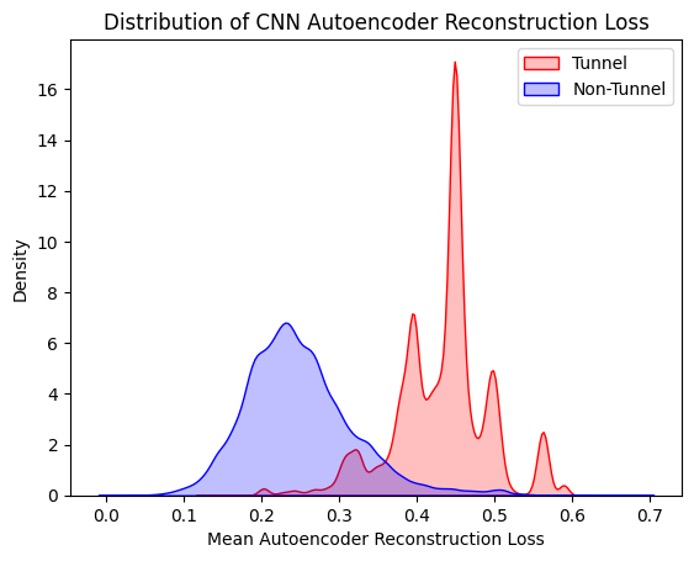
Figure 2. KDE plot for CNN autoencoder reconstruction loss
Word Segmentation-Based Feature Extraction
The majority of legitimate prefixes use natural language words, whereas tunneling prefixes often employ hex, base32 or similar encodings that result in a larger number of word segments. We employ a cost-based word segmentation technique that segments strings into words found in language dictionaries to derive segmentation-based features. For example, the string “facebooksecurity” segments into [“face”, “book”, “security”], while an encoded string such as “youjf34gwid86fih” segments into [“you”, “j”, “f”, “34”, “g”, “w”, “id”, “86”, “f”, “i”, “h”] since no dictionary words match the encoded content.
Using this segmentation technique, we derive multiple features including the ratio of segment count to query name length. We observe that tunneling domains exhibit significantly higher segment-to-length ratios due to their encoded nature—random or encrypted data breaks down into many small, unrecognizable fragments rather than coherent dictionary words. This creates a highly discriminative feature where tunnel prefixes consistently produce much higher ratios compared to legitimate domains.
Table 4 demonstrates this discriminative power through concrete examples. The benign domain “facebooksecurity” achieves a low segment ratio of 0.19 (3 segments/16 characters), while the tunnel prefix “youjf34gwid86can” produces a much higher ratio of 0.69 (11 segments/16 characters). This substantial difference in segment ratios provides a reliable signal for distinguishing between legitimate domain patterns and encoded tunneling data.
| Type | Prefix | Segments | Segment Size (SS) | Prefix Length (PL) | Segment Ratio (SS/PL) |
|---|---|---|---|---|---|
| Benign | facebooksecurity | [“face”, “book”, “security”] | 3 | 16 | 0.19 |
| Tunnel | youjf34gwid86fih | [“you”, “j”, “f”, “34”, “g”, “w”, “id”, “86”, “f”, “i”, “h”] | 11 | 16 | 0.69 |
| Table 4. Word segmentation comparison for tunnel vs. benign domains | |||||
Results—Classifier Performance
We evaluated our approach using multiple classification algorithms to establish comprehensive performance baselines. Table 5 presents the performance comparison between Random Forest and Logistic Regression classifiers across both query-level and domain-level metrics.
| Metrics | Random Forest Classifier Score (%) | Logistic Regression Classifier Score (%) |
|---|---|---|
| Query-Level Performance | ||
| Accuracy | 99.76 | 91.01 |
| Recall | 99.51 | 98.13 |
| Precision | 99.92 | 83.66 |
| F1 | 99.71 | 90.32 |
| Domain-Level Performance | ||
| SLD Recall | 98.69 | 95.42 |
| SLD Precision | 94.97 | 34.76 |
| SLD F1 | 96.79 | 50.96 |
| Table 5. Random Forest and Logistic Regression classifier performance | ||
The Random Forest classifier demonstrates superior performance across all metrics, achieving an F1 score of 99.71 percent at the query level and 96.79 percent at the domain level. While Logistic Regression maintains competitive recall (98.13 percent query-level, 95.42 percent domain-level), it performs with significantly lower precision, particularly at the domain level (34.76 percent), resulting in a substantially lower domain-level F1 score of 50.96 percent.
The domain-level metrics are particularly important for operational deployment, as they reflect the classifier’s ability to correctly identify tunneling domains rather than individual queries. These metrics are calculated by aggregating results at the SLD level: domain-level recall measures the number of unique tunnel SLDs correctly identified divided by the total number of unique tunnel SLDs in the test set, while domain-level precision calculates the number of unique tunnel SLDs correctly identified divided by the total number of unique SLDs flagged as tunnels. This approach provides a more operationally relevant view than query-level metrics, as we typically need to block entire domains rather than individual queries. This is why we are particularly worried about precision, as blocking at the SLD level can add significant risk of blocking a domain that is potentially useful to our customers. The Random Forest’s strong domain-level precision (95 percent) indicates effective reduction of false positive alerts, which is crucial for practical cybersecurity applications. Equally important, the model achieves exceptional domain-level recall (99 percent), demonstrating its ability to detect nearly all tunneling domains with minimal false negatives. This high recall ensures that malicious DNS tunneling activities are rarely missed, providing comprehensive threat coverage.
The emphasis on maximizing recall is strategically designed for our multi-stage detection architecture. In our systems, the primary classifier serves as a comprehensive detection layer that captures potential threats with minimal risk of missing genuine attacks, while subsequent validation processes systematically filter out false positives through additional verification mechanisms and threat intelligence correlation. Additionally, our defense-in-depth approach ensures that any tunnels potentially missed by this classifier can still be detected by our complementary DNS tunnel detection systems, providing multiple layers of protection against evasive tunneling techniques. This approach prioritizes comprehensive threat detection over initial precision, recognizing that missing a genuine DNS tunnel poses significantly greater security risks than flagging legitimate traffic for further analysis. Through these secondary validation stages, the system ensures that false positives are reduced, allowing only likely malicious DNS tunnels to trigger final alerts and automated response actions.
The combination of strong recall and precision scores at the domain level indicate the Random Forest model is capable of performing operational DNS tunnel detection, where maintaining thorough threat coverage while minimizing analyst workload is essential for scalable cybersecurity operations.
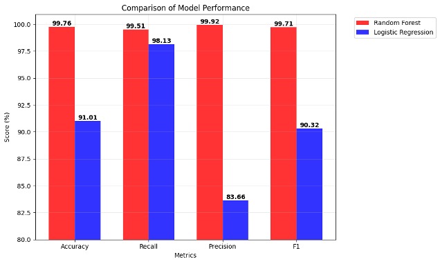
Figure 4. Comparison of query-level model performance
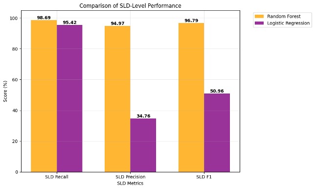
Figure 5. Comparison of SLD-level model performance
Evaluation of Novel Features: Measuring Impact Through Feature Removal
To evaluate the contribution of our novel features—autoencoder reconstruction loss and word segmentation ratios—we conducted an ablation study by training the Random Forest classifier with and without these enhancements. This analysis quantifies the direct impact of our proposed features on model performance.
As shown in Figure 6, the removal of novel features results in substantial performance degradation across all metrics. Most notably, SLD-level precision drops significantly from 95 percent to 86 percent when novel features are excluded, while SLD-level recall decreases from 99 percent to 98 percent. The F1 score similarly declines from 97 percent to 92 percent, demonstrating the critical importance of these features for effective tunnel detection.
The precision improvement is particularly significant given our operational context, where the system processes DNS traffic at the scale of billions of events per day. Even a modest increase in precision translates to a substantial reduction in false positive alerts, potentially eliminating thousands of incorrect flags daily. This reduction directly impacts secondary validation tasks and system efficiency, making the novel features essential for practical deployment. Furthermore, the maintained high recall ensures that genuine threats are not missed despite the improved precision, validating the effectiveness of our feature engineering approach.
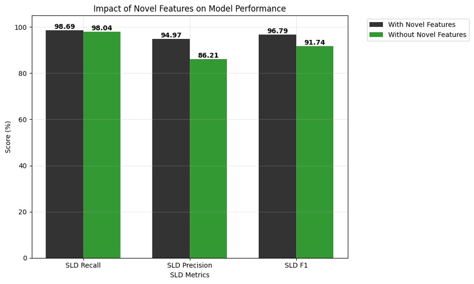
Figure 6. Impact of novel features on model performance
Real-Time Implementation
In our production platform, we create feature summaries and execute the model in near– real time to process billions of DNS queries daily. Our high-throughput data processing infrastructure enables us to detect potential tunneling activity within seconds of occurrence.
Following the primary detection, secondary validation processes are performed to enhance precision and reduce false positives. These include:
- Allowlist Validation: Removing known benign tunneling applications such as antivirus software, security tools and legitimate update mechanisms
- Infrastructure Analysis: Examining name servers, registrars and hosting providers associated with flagged SLDs
- Behavioral Correlation: Cross-referencing with threat intelligence and historical patterns
The secondary validation layer operates as a scalable microservice architecture, providing resilient processing of flagged domains. After completing both primary detection and secondary validation, the system performs final actions including alerting, blocking or forwarding to security teams for investigation.